
A necessary (but not sufficient) condition for numerical stability is the Courant-Freidrich-Lewy condition which restricts the maximum timestep:
\[\begin{align} \Delta t \leq \frac{ \Delta x }{ c } \end{align}\]where \(\Delta x\) is the grid spacing and \(c\) the characteristic velocity of the flow. This is easy to calculate if the grid is regular, but what if your grid is a discretized slice of the ocean, and consequently looks something like this:
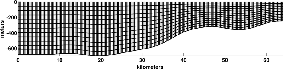
in which each of the tiny boxes themselves represent a 15 x 15 mesh of Gauss-Lobatto-Legendre quadrature points. This is the case in a high-order element-based code like the spectral multi-domain penalty method, and the computation of the CFL condition (and namely the local deformation \(\Delta x\)) is not quite so straightforward.
Computing the grid spacing in the master element
Call the coordinates on the master element \((\eta,\xi)\), and noting that there are \(n\) GLL points in each direction, these coordinates are vectors \(\eta,\xi \in \mathbb{R}^{n^2}\). The mapping functions that define the physical grid are defined on each element as \(x_k = x_k(\eta,\xi)\) and \(z_k = z_k(\eta,\xi)\). Call the collection of all of these maps \(x\) and \(z\) (drop the subscripts. What we want, for computing the CFL condition, is some measure of \(\Delta x\) and \(\Delta z\), the spacing between grid points in a deformed domain like the one shown above.
Probably there are many ways to do this, but the one I chose was to make use of the fact that it is easy to get a measure of \(\Delta \eta\) and \(\Delta \xi\) on the master element. For example for the one-dimensional case, compute \(\Delta \eta \in \mathbb{R}^n\) using a centered finite difference approximation:
\[\begin{align} (\Delta \eta )_j &= \eta_{j+1} - \eta_{j-1} \end{align}\]for \(j = 2, 3, \cdots, n - 1\), with \((\Delta \eta)_1 = \eta_2 - \eta_1\) and \((\Delta \eta)_n = \eta_n - \eta_{n-1}\). The same idea extends to two-dimensions and computing \(\Delta\xi\) along with \(\Delta\eta\).
Computing the spacing everywhere in grid
Remember that we can easily compute derivatives in \(\eta\) and \(\xi\); that is the whole point of defining these coordinates, to be able to use them in constructing spectral differentiation matrices and computing numerical derivatives. Using the mapping functions \(x_k\) and \(z_k\) we can then use the chain rule to write the grid spacing on each element as (again dropping the \(k\) in the subscript) as functions of derivatives in \((\eta,\xi)\) coordinates:
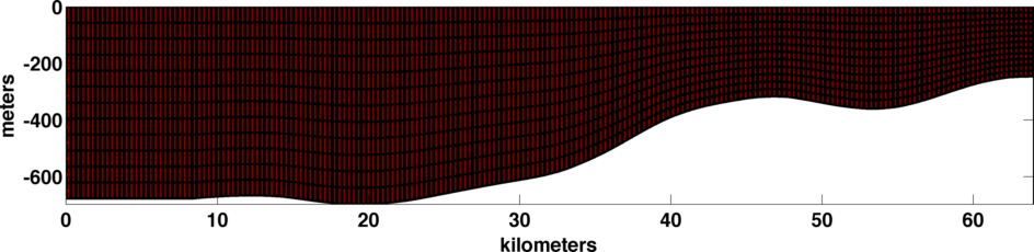
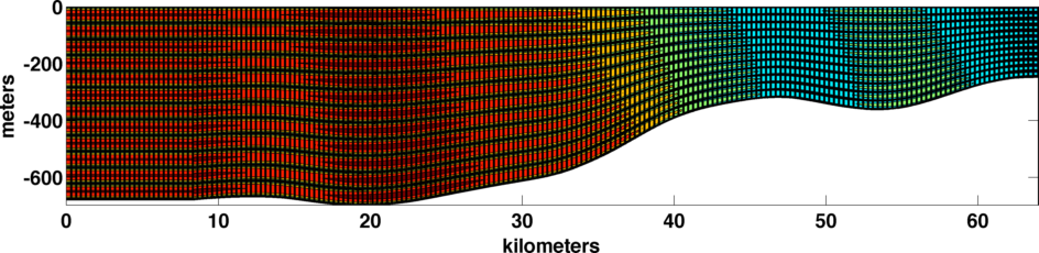
\[\begin{align} \Delta x &= \frac{\partial x}{\partial \eta } \Delta \eta + \frac{\partial x}{\partial \xi} \Delta \xi \\ \Delta z &= \frac{\partial z}{\partial \eta } \Delta \eta + \frac{\partial z}{\partial \xi} \Delta \xi. \end{align}\]These quantities are shown in the figures below; the \(\Delta x\) function is basically constant and so is kind of boring (the grid is uniformly spaced in the horizontal), but the \(\Delta z\) function has some interesting character as the bathymetry slopes and shallows.
Computing a maximum time-step
Using these two quantities, \(\Delta x\) and \(\Delta z\), we can define the maximum time-step allowed in the simulation as
\[\begin{align} \Delta t _{max} = \min_{(x,z)\in \Omega} \min \left\{ \frac{\Delta x(x,z)}{u_x(x,z)}, \frac{\Delta z(x,z)}{u_z(x,z)} \right\} \end{align}\]which ensures that we are satisfying \(\Delta t \leq \Delta x / u_x\) and \(\Delta t \leq \Delta z / u_z\) everywhere in the domain \(\Omega\). All of the quantities on the right hand side of the above are computable, and are defined above.
Example: shoaling internal wave
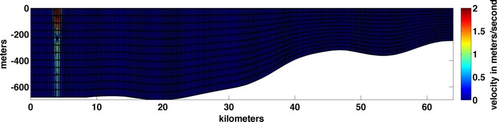
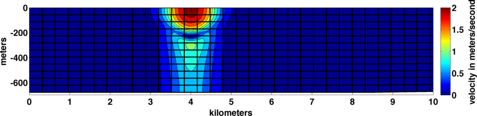
Setting an initial velocity field that represents a propagating internal wave (as shown in the two pictures above), we can compute the quantity \(\Delta t(x,z)\):
\[\begin{align} \Delta t(x,z) = \min \left\{ \frac{\Delta x(x,z)}{u_x(x,z)}, \frac{\Delta z(x,z)}{u_z(x,z)} \right\}. \end{align}\]The minimum value of this function is the maximum allowable time-step as determined by the CFL condition. Of course, this function is not constant, and so parts of the grid will have too fine a time-step (i.e. if there is nothing going on in the velocity field there). But this inefficiency is inescapable since the grid has to advance in time together, and so we have to take the minimum value over the whole grid. Corresponding to the the internal wave field shown above, \(\Delta t(x,z)\) is shown in the two figures below.
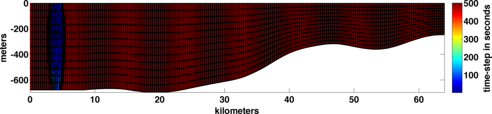
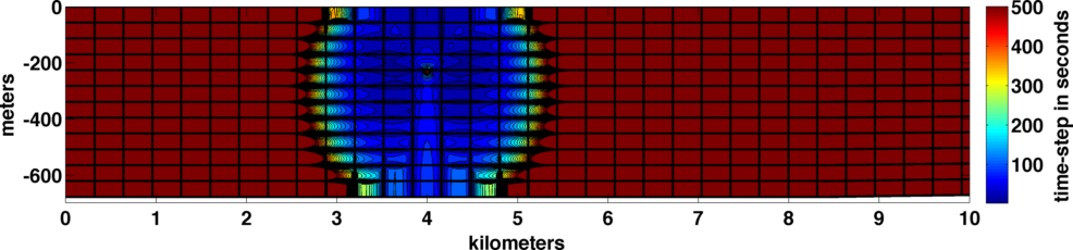
For this particular field, the maximum time-step allowed, as computed by this method, turns out to be \(\Delta t_{max} \approx 1.6\) seconds, and is governed by a tiny region in the middle of wave field near an element boundary. This makes sense, near the center of the wave the velocity is the highest, and near an element boundary the grid spacing is the most fine.
Finally, what if we skipped this computation and instead used a heuristic to estimate the time-step? If instead of doing the above computation, we were to establish a minimum time-step by guessing an average grid spacing and the using the maximum velocity, we would get a very different (and too large) answer of \(\Delta t_{max} \approx 6.3\) seconds. If we attempted to be more conservative and calculated the difference between closest two grid points and divided by the maximum velocity in the grid, we’d get a far too conservative answer of \(\Delta t_{max} \approx 3 \times 10^{-4}\) seconds. The point being: don’t skip this computation.